Step 1: Introduction & Problem Statement
Can a machine learning model hear the difference between the swinging 60s and the electronic 80s just by analyzing audio features? How does music's 'sound' evolve across decades? This project dives into that question by building and optimizing a Deep Neural Network (DNN).
My journey begins with the following:
- Dataset: The YearPredictionMSD dataset from the UCI Machine Learning Repository, containing 515,000+ songs described by 90 audio features.
- Goal: Transform this regression challenge into a 10-class classification problem – predicting the decade of release, from the 1920s up to the 2010s.
- Tool: I'll use PyTorch, a powerful deep learning framework, to build, train, and meticulously optimize my DNN model.
Let me explore how I tackled this challenge, step by step.
Step 2: Understanding the Soundscape - Data Exploration & Prep
Before training any model, understanding the data is crucial. I started by transforming the raw year data and exploring the characteristics of the audio features.
Decade Binning
The first step, handled in src/data_processing.py, was converting the continuous 'Year' variable into discrete decade labels. I mapped years into 10 bins, representing the 1920s (label 0) through the 2010s (label 9).
Class Imbalance
Visualizing the distribution of songs across these new decade labels immediately revealed a significant challenge: class imbalance.
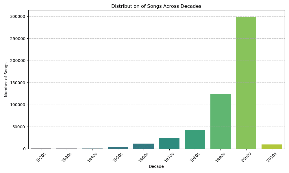
This imbalance necessitated using stratified splitting for my train (70%), validation (15%), and test (15%) sets to ensure each decade is proportionally represented across all subsets.
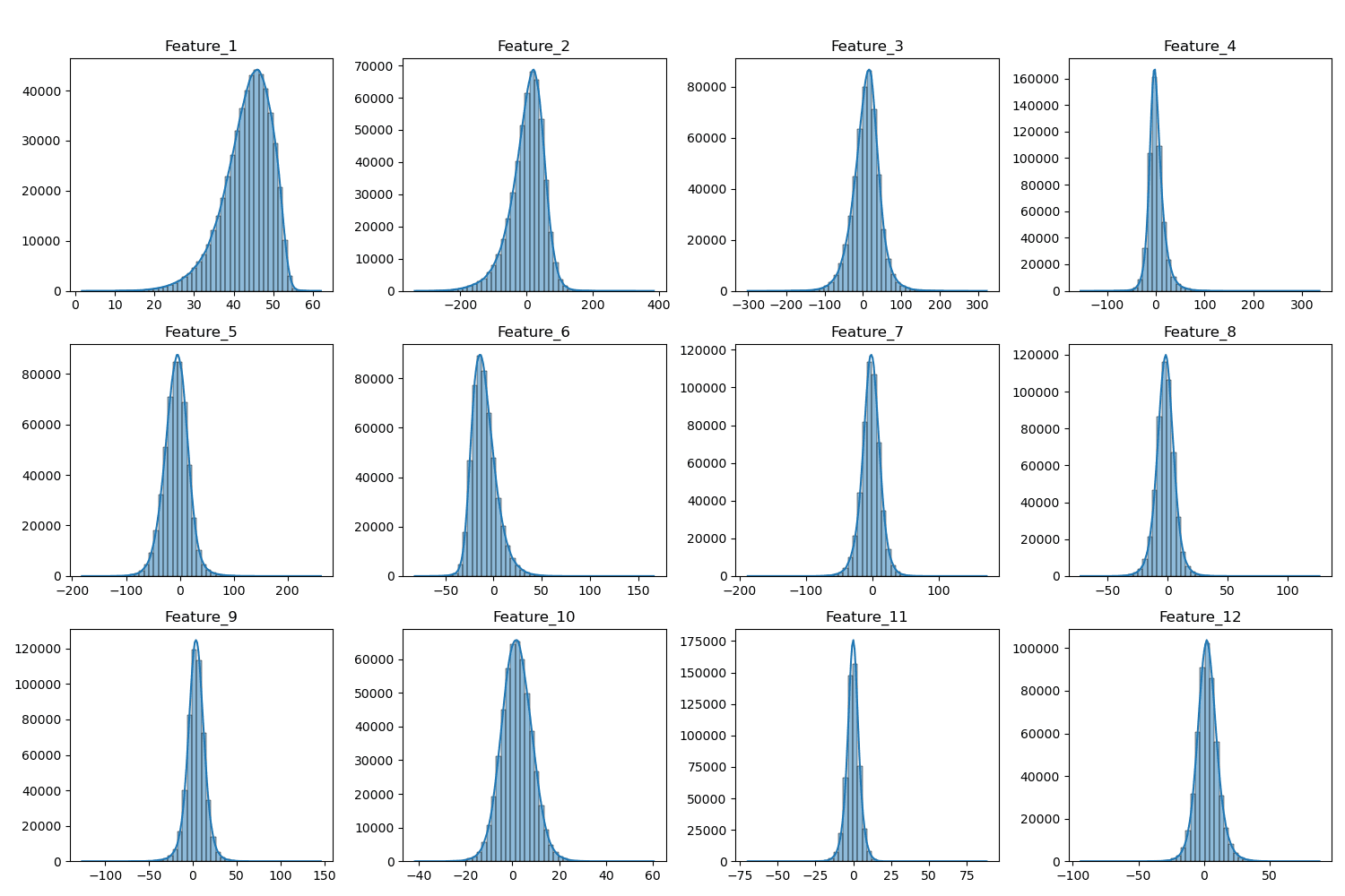
Feature Insights
I examined the distributions of the first 12 features (timbre averages) using histograms and box plots. These plots showed varying distributions – some roughly normal, others skewed – and highlighted the presence of potential outliers.
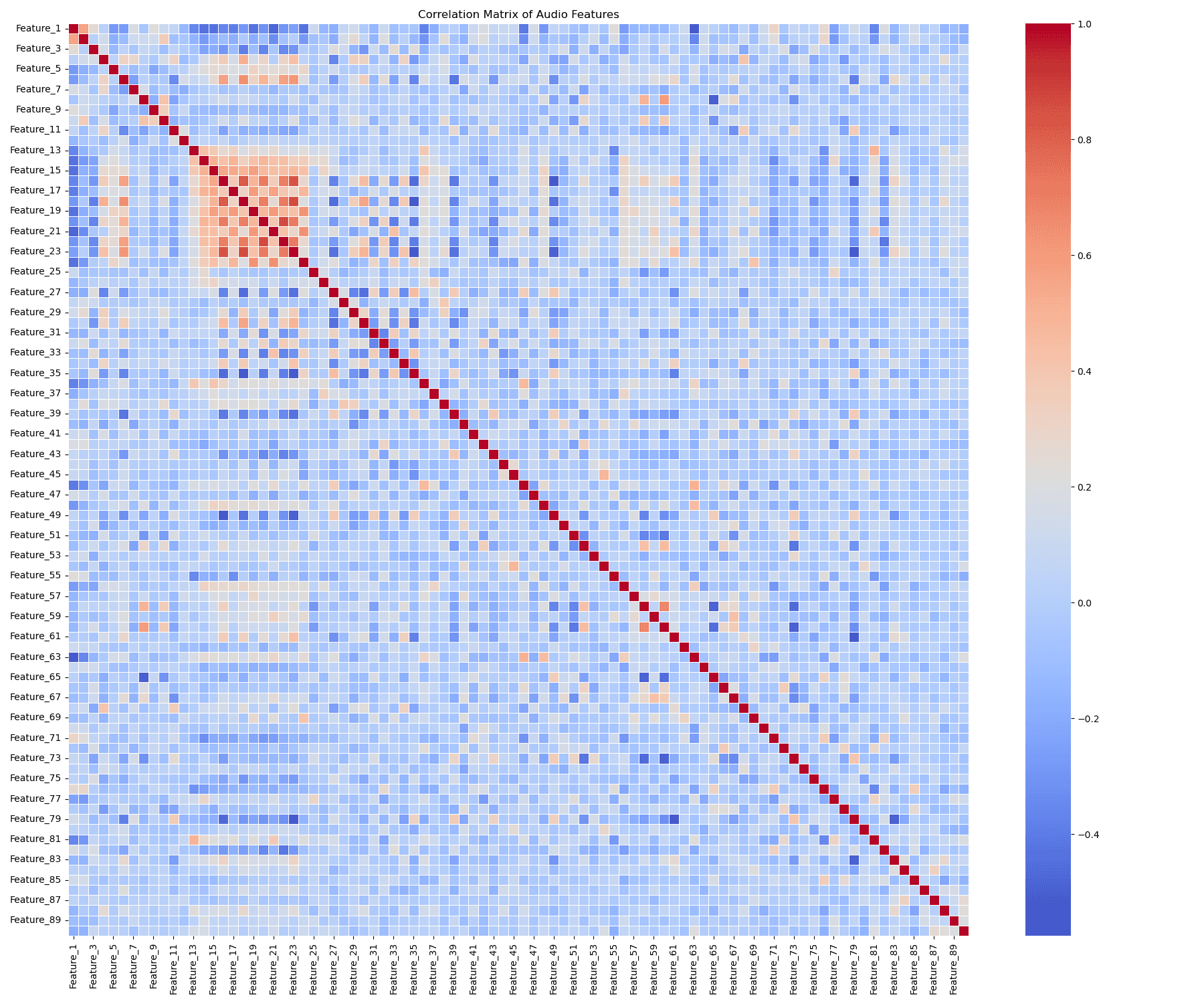
Correlations
A heatmap of feature correlations indicated moderate relationships within certain feature groups (like the timbre averages or covariance features), suggesting some inherent structure related to the audio properties.
Step 3: Setting the Stage - Baseline Model Performance
With prepared data, the next step was to establish baseline performance using simple DNN architectures. I tested three architectures:
- Model_1 (128x128): Two hidden layers with 128 neurons each. (29k params)
- Model_2 (256x256): Two hidden layers, but wider with 256 neurons each. (92k params)
- Model_3 (256x128x64): Three hidden layers with decreasing width. (65k params)
| Architecture | Final Val Loss | Final Val Accuracy | Training Time |
|---|---|---|---|
| Model_1 (128x128) | 1.4841 | 0.5802 | 1.53s |
| Model_2 (256x256) | 1.2711 | 0.5802 | 1.40s |
| Model_3 (256x128x64) | 1.3519 | 0.5802 | 1.47s |
Model_2 (256x256) consistently achieved the lowest validation loss, so it was selected as the baseline architecture for systematic optimization.
Step 4: Tuning the Instrument - Systematic Optimization
Having chosen Model_2 as my base, I embarked on a systematic optimization process. My strategy was to tune hyperparameters and test components sequentially, carrying forward the best setting from each stage.
1. Learning Rate Search
We used the torch-lr-finder library to perform an LR range test. The model was trained for one epoch with the LR exponentially increasing, and the loss was plotted against the LR.
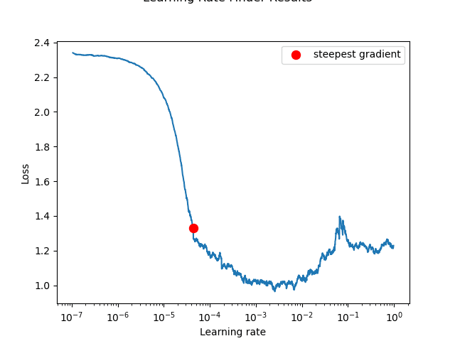
Selected Optimal Learning Rate: 0.001
2. Weight Decay Tuning
We employed 5-Fold Cross-Validation on the training set. For each Weight Decay value, Model_2 was trained 5 times (10 epochs each).
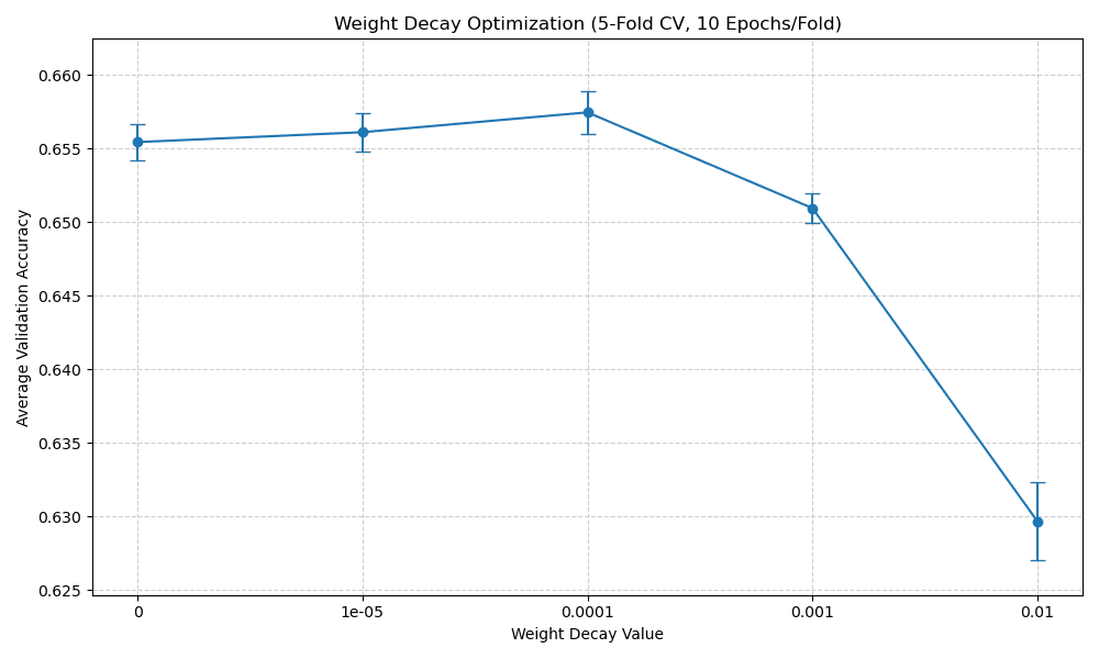
Selected Optimal Weight Decay: 0.0001
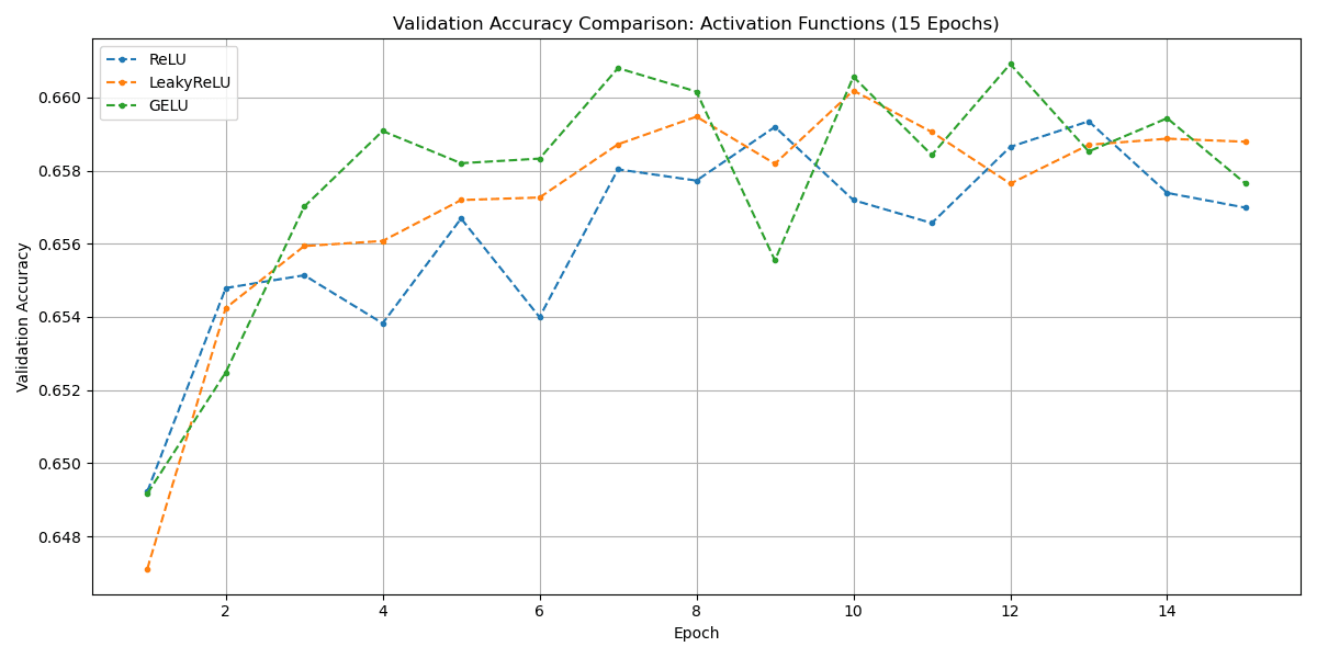
3. Component Sweeps
We tested variations of core neural network components:
Initialization: Default (Kaiming Uniform), Xavier Uniform, Kaiming Normal were tested. Differences were minimal, with Default performing marginally best.
Activation: ReLU, LeakyReLU, and GELU were compared. GELU achieved the highest peak validation accuracy (0.6609).
Normalization: None, BatchNorm1d, and LayerNorm were tested. Surprisingly, No Normalization performed best in this setup.
Optimizer: Adam, SGD (momentum=0.9), and RMSprop were compared. RMSprop achieved the highest peak accuracy (0.6617).
Step 5: The Performance - Final Model Training & Results
With all components optimized, I assembled the final configuration:
Final Optimized Configuration:
- • Architecture: Model_2 (256x256)
- • Initialization: Default (Kaiming Uniform)
- • Activation: GELU
- • Normalization: None
- • Optimizer: RMSprop
- • Learning Rate: 0.001
- • Weight Decay: 0.0001
Final Training Run
This final model was trained on the entire training dataset for 15 epochs, using the validation set to monitor progress.
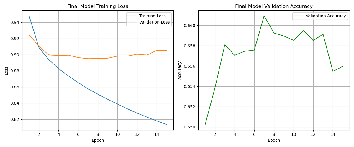
Test Set Evaluation
The ultimate measure of success is performance on the unseen test set:
Step 6: Key Takeaways - Lessons from the Tuning Process
This journey from raw data to an optimized DNN yielding 66.05% accuracy on a challenging, imbalanced decade classification task highlighted several valuable lessons:
- Systematic > Haphazard
Tuning hyperparameters and components sequentially, carrying forward the best, provides clearer insights than changing multiple things at once.
- Data is Foundational
Addressing data issues like class imbalance early (with stratified splitting) and applying appropriate preprocessing (like scaling) are critical first steps.
- Informed Tuning Beats Guesswork
Tools like LR Finder for learning rates and techniques like K-Fold CV for regularization parameters provide data-driven starting points and validation.
- Context is King
The "best" component isn't universal. While GELU and RMSprop showed slight advantages here, optimal choices depend heavily on the dataset, architecture, and training duration.
- The Test Set Reigns Supreme
Validation sets guide optimization, but the final, untouched test set provides the only unbiased measure of how well the model generalizes.
Project Resources & Downloads
data_processing.py
Data loading, preprocessing, and tensor conversion
models.py
DNN architectures and model components
Jupyter Notebooks
Interactive notebooks with code and analysis
PDF Reports
Rendered notebooks with outputs and visualizations
Key Takeaway
Building production ML models isn't about finding a silver bullet—it's about systematic experimentation and rigorous validation.
The journey from 58% baseline to 66% test accuracy demonstrates that small, informed decisions compound into significant improvements.
