Step 1: Introduction & Problem Statement 1 min read
Can a machine learning model hear the difference between the swinging 60s and the electronic 80s just by analyzing audio features? How does music's 'sound' evolve across decades? This project dives into that question by building and optimizing a Deep Neural Network (DNN).
My journey begins with the following:
- Dataset: The YearPredictionMSD dataset from the UCI Machine Learning Repository, containing 515,000+ songs described by 90 audio features (like timbre averages and covariances). Its original task is predicting the exact release year.
- Goal: Transform this regression challenge into a 10-class classification problem – predicting the *decade* of release, from the 1920s up to the 2010s.
- Tool: I'll use PyTorch, a powerful deep learning framework, to build, train, and meticulously optimize my DNN model.
Let me explore how I tackled this challenge, step by step.
Step 2: Understanding the Soundscape - Data Exploration & Prep 2 min read
Before training any model, understanding the data is crucial. I started by transforming the raw year data and exploring the characteristics of the audio features.
Decade Binning
The first step, handled in src/data_processing.py, was converting the continuous 'Year' variable into discrete decade labels. I mapped years into 10 bins, representing the 1920s (label 0) through the 2010s (label 9).
Class Imbalance
Visualizing the distribution of songs across these new decade labels immediately revealed a significant challenge: class imbalance.
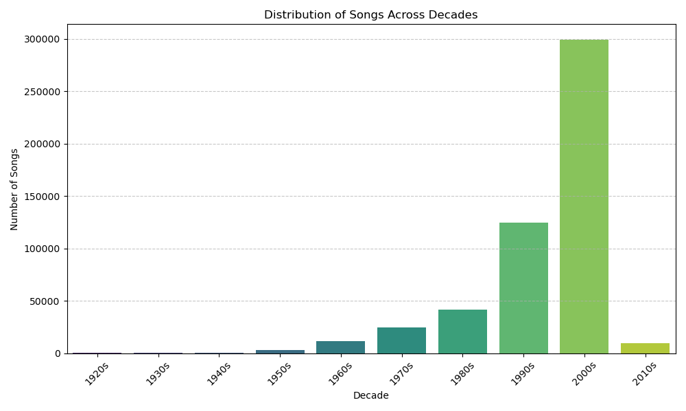
The dataset is heavily dominated by songs from the 1990s (label 7) and 2000s (label 8).
This imbalance necessitated using stratified splitting for my train (70%), validation (15%), and test (15%) sets to ensure each decade is proportionally represented across all subsets.
Feature Insights
I examined the distributions of the first 12 features (timbre averages) using histograms and box plots. These plots, generated in my exploration notebook, showed varying distributions – some roughly normal, others skewed – and highlighted the presence of potential outliers.
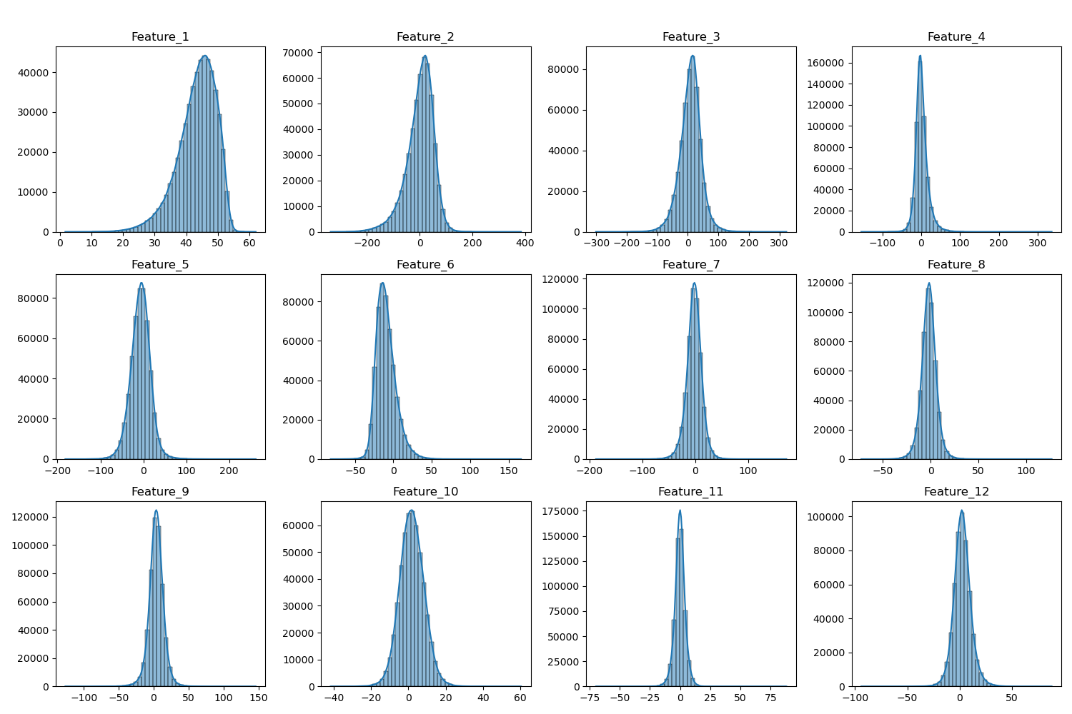
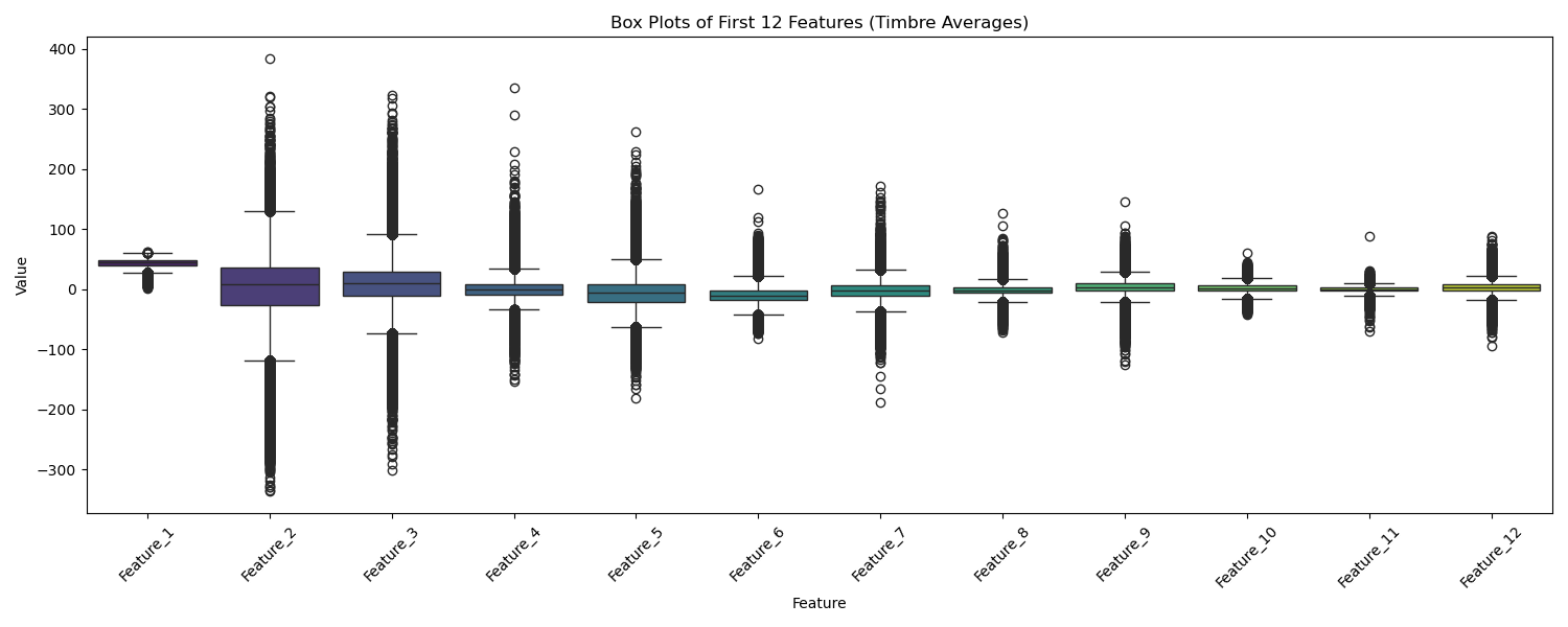
Histograms and box plots revealed diverse feature distributions and potential outliers.
Correlations
A heatmap of feature correlations indicated moderate relationships within certain feature groups (like the timbre averages or covariance features), suggesting some inherent structure related to the audio properties. However, no extremely high correlations (>0.95) were immediately apparent, reducing concerns about major feature redundancy.
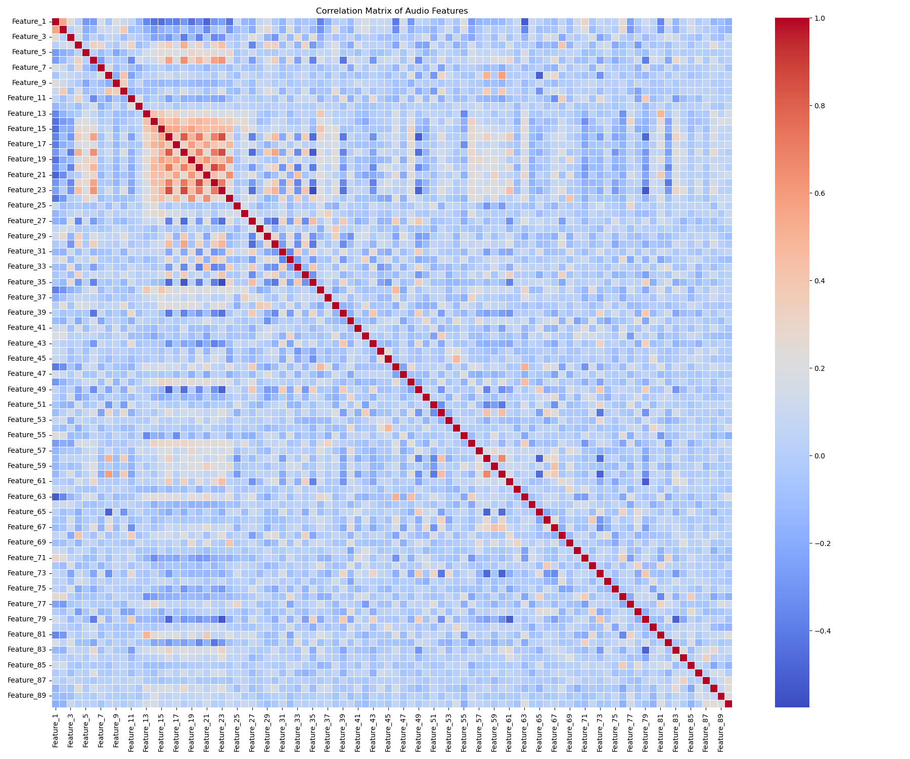
Moderate correlations exist, particularly within feature blocks.
Handling Outliers and Scaling
The box plots clearly showed outliers. While several strategies exist (RobustScaler, clipping, transformations), we decided to initially proceed using StandardScaler. This standardizes features to have zero mean and unit variance. It's sensitive to outliers, but deep learning models (especially with techniques like Batch Normalization, tested later) can sometimes handle them robustly. We fit the scaler *only* on the training data to prevent data leakage and applied it to all splits.
Final Touches
Finally, the preprocessed and scaled data was converted into PyTorch tensors, ready for model training.
Step 3: Setting the Stage - Baseline Model Performance 1 min read
With prepared data, the next step was to establish baseline performance using simple DNN architectures. This helps gauge the task's difficulty and provides a benchmark for optimization efforts. I tested three architectures defined in src/models.py:
- Model_1 (128x128): Two hidden layers with 128 neurons each. (29k params)
- Model_2 (256x256): Two hidden layers, but wider with 256 neurons each. (92k params)
- Model_3 (256x128x64): Three hidden layers with decreasing width. (65k params)
All baseline models initially used the ReLU activation function.
Initial Run & Comparison
I performed a very short training run (15 mini-batches) for each model using the Adam optimizer (LR=0.001) and evaluated performance on the validation set every 5 batches (details in notebooks/2_Initial_Model_Runs.ipynb).
Note: Due to the limited nature of this initial run (only 15 batches), the plots primarily show initial learning trends rather than converged performance. Explicit comparison plots weren't saved, but the validation metrics were logged.
| Architecture | Final Val Loss (15 batches) | Final Val Accuracy (15 batches) | Training Time (s) |
|---|---|---|---|
| Model_1 (128x128) | 1.4841 | 0.5802 | 1.53 |
| Model_2 (256x256) | 1.2711 | 0.5802 | 1.40 |
| Model_3 (256x128x64) | 1.3519 | 0.5802 | 1.47 |
Selection: Model_2
Although all models reached the same validation accuracy plateau (0.5802) very quickly within these 15 batches, Model_2 (256x256) consistently achieved the lowest validation loss at each evaluation point. This suggested it might have a slight edge in initial learning dynamics or capacity for this task. Therefore, Model_2 was selected as the baseline architecture for the subsequent systematic optimization phase.
Step 4: Tuning the Instrument - Systematic Optimization of Model_2 5 min read
Having chosen Model_2 as my base, I embarked on a systematic optimization process, documented in notebooks/3_Optimization_Experiments.ipynb. My strategy was to tune hyperparameters and test components sequentially, carrying forward the best setting from each stage.
-
Learning Rate Search
- Why: Find an optimal learning rate (LR) for efficient convergence. Too high, and training diverges; too low, and it's slow.
- How: We used the
torch-lr-finderlibrary to perform an LR range test. The model was trained for one epoch with the LR exponentially increasing, and the loss was plotted against the LR. We looked for the LR corresponding to the steepest drop in loss before it started increasing. A short 5-epoch verification run confirmed the chosen LR's stability. - Result:
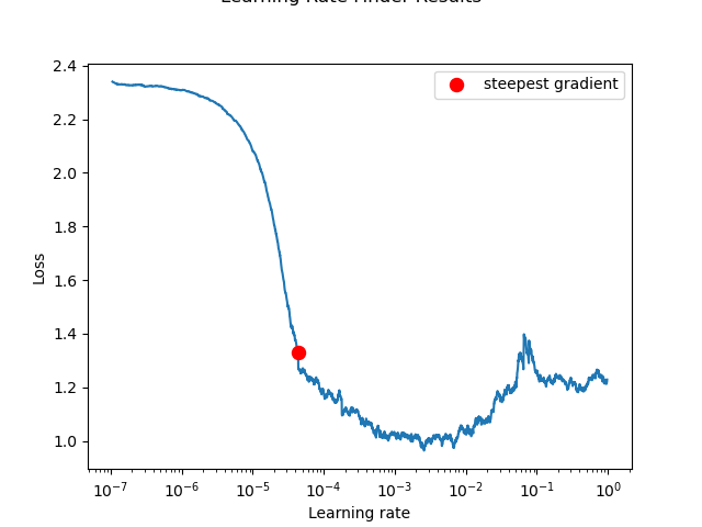
LR Finder plot and the 5-epoch verification confirmed stable learning.
The plot suggested an optimal LR around 0.001. Verification confirmed stable learning.
Selected Optimal LR: 0.001
-
Weight Decay Tuning
- Why: Apply L2 regularization (Weight Decay, WD) to penalize large weights and potentially improve generalization by preventing overfitting.
- How: We employed 5-Fold Cross-Validation on the training set. For each WD value in
[0, 1e-5, 1e-4, 1e-3, 1e-2], Model_2 (with LR=0.001) was trained 5 times (10 epochs each), using a different fold for validation each time. Average validation accuracy across the folds determined the best WD. - Result:
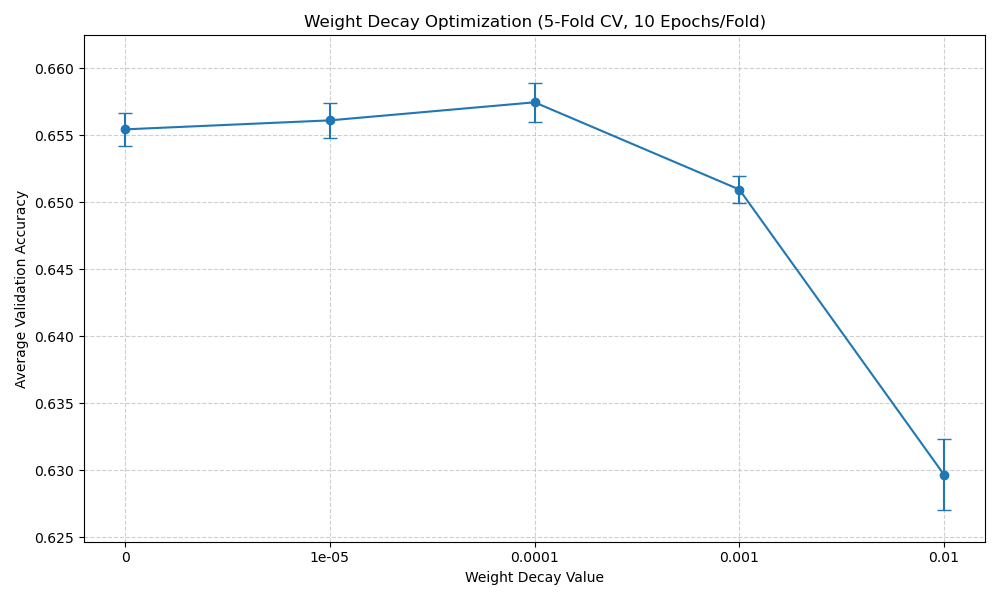
A small amount of regularization (WD=0.0001) yielded the best average validation accuracy.Weight Decay Avg Val Acc Std Val Acc 0 0.6555 0.0012 1e-05 0.6561 0.0013 0.0001 0.6575 0.0014 0.001 0.6510 0.0010 0.01 0.6297 0.0026
Selected Optimal Weight Decay: 0.0001
-
Component Sweeps
- Why: Evaluate the impact of different core neural network components.
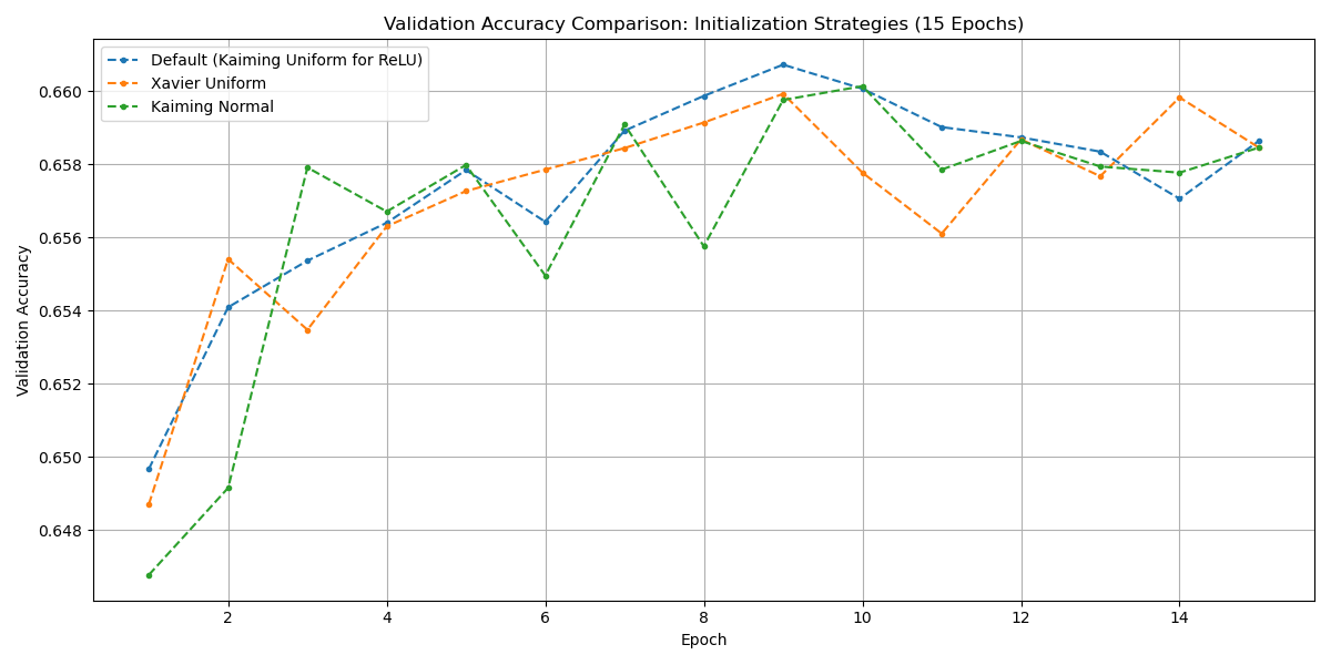
- How: We tested variations of one component type at a time (Initialization, Activation, Normalization, Optimizer), training Model_2 (with optimal LR=0.001 and WD=0.0001) for 15 epochs for each variation. The component yielding the highest *peak* validation accuracy during its test was selected.
- Result:
Initialization: Default (Kaiming Uniform for ReLU), Xavier Uniform, Kaiming Normal were tested. Differences were minimal, with Default performing marginally best.
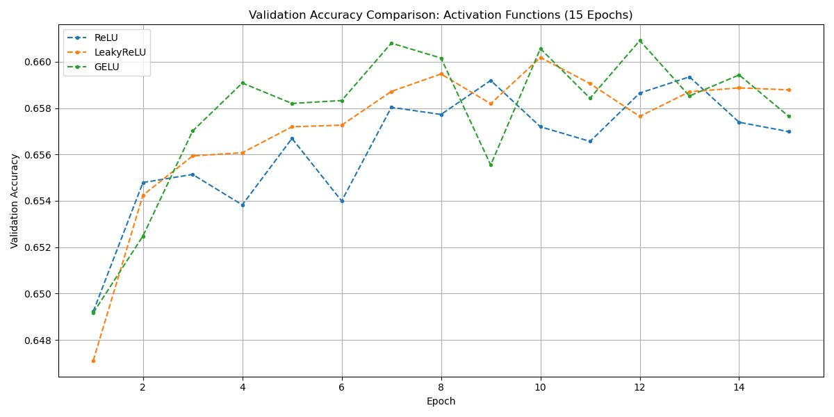
Activation: ReLU, LeakyReLU, and GELU were compared. GELU achieved the highest peak validation accuracy (0.6609).
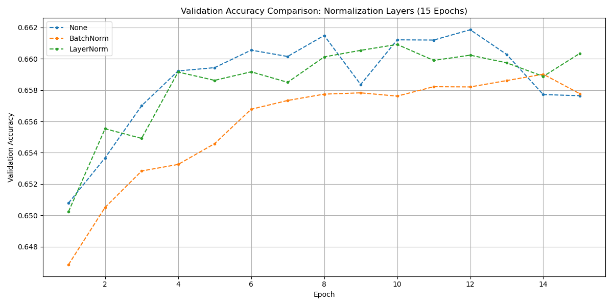
Normalization: None, BatchNorm1d, and LayerNorm were tested (requiring a flexible `models.py`). Surprisingly, *No Normalization* performed best (peak accuracy 0.6619) in this 15-epoch test setup. Normalization might become more beneficial with deeper networks or longer training.
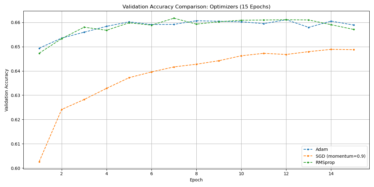
Optimizer: Adam, SGD (with momentum=0.9), and RMSprop were compared, using the optimal LR and WD. RMSprop achieved the highest peak accuracy (0.6617).
Selected Components: Default Init, GELU Activation, No Normalization, RMSprop Optimizer.
Step 5: The Performance - Final Model Training & Results 1 min read
With all components optimized, I assembled the final configuration:
Final Optimized Configuration:
- Architecture: Model_2 (256x256)
- Initialization: Default (Kaiming Uniform for ReLU)
- Activation: GELU
- Normalization: None
- Optimizer: RMSprop
- Learning Rate: 0.001
- Weight Decay: 0.0001
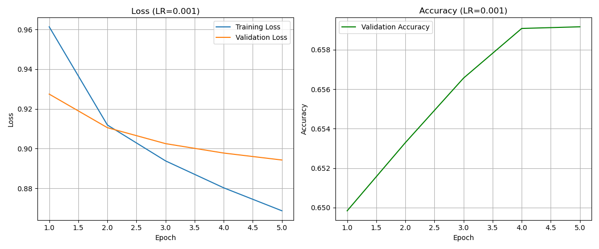
Final Training Run
This final model was trained on the *entire* training dataset for 15 epochs, using the validation set to monitor progress. I included a basic early stopping check (stop if validation loss doesn't improve for 5 epochs), though it wasn't triggered within the 15 epochs.
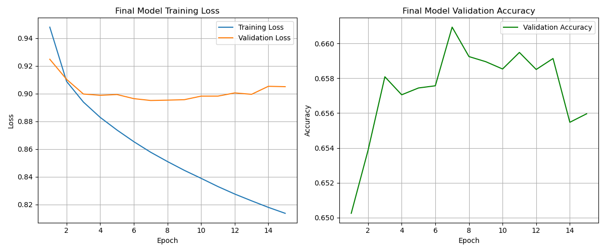
The final model's learning curves over 15 epochs.
Test Set Evaluation
The ultimate measure of success is performance on the unseen test set. My fully optimized model achieved:
Final Test Loss: 0.8993
Final Test Accuracy: 66.05%
The state dictionary of this final, optimized model was saved to results/models/final_optimized_model.pth for future use or deployment.
Step 6: Key Takeaways - Lessons from the Tuning Process 1 min read
This journey from raw data to an optimized DNN yielding 66.05% accuracy on a challenging, imbalanced decade classification task highlighted several valuable lessons:
- Systematic > Haphazard: Tuning hyperparameters and components sequentially, carrying forward the best, provides clearer insights than changing multiple things at once.
- Data is Foundational: Addressing data issues like class imbalance early (with stratified splitting) and applying appropriate preprocessing (like scaling) are critical first steps.
- Informed Tuning Beats Guesswork: Tools like LR Finder for learning rates and techniques like K-Fold CV for regularization parameters (Weight Decay) provide data-driven starting points and validation.
- Context is King: The "best" component isn't universal. While GELU and RMSprop showed slight advantages *here*, normalization layers (often crucial) didn't help in *this specific 15-epoch setup*. Optimal choices depend heavily on the dataset, architecture, and training duration.
- The Test Set Reigns Supreme: Validation sets guide optimization, but the final, untouched test set provides the only unbiased measure of how well the model generalizes to new, unseen data.
While further improvements might be possible, this structured approach provides a solid methodology for building and refining deep learning models effectively.